Getting Started
AlphaD3M is integrated with Jupyter Notebooks. The Jupyter notebooks provide an interactive computing environment where you can generate models using AlphaD3M, and explore them using PipelineProfiler which is an interactive visualization aimed at producing detailed visualizations of end-to-end machine learning pipelines. AlphaD3M has two main components: model generation and model exploration.
Model Generation
The model generation component provides methods to search, train, test, and score pipelines.
First, import the class AutoML. If you plan to use AlphaD3m via Docker/Singularity, use: DockerAutoML or SingularityAutoML classes.
[1]:
from alphad3m import AutoML
Then, search for pipelines using the imported class. AutoML receives the output path to be used.
To perform the search of pipelines, we need to call search_pipelines. This call needs the following parameters: the training dataset; the maximum running time (time_bound) in minutes; the variable to predict (target); the metric to be used (metric); and the keywords that describe the task to be solved (task_keywords). The time_bound controls how long the search can take and control the use of computational resources. Note that longer running times may lead to more
accurate solutions since the system will have more time to try and evaluate more candidate solutions for the problem.
The 185_baseball_MIN_METADATA dataset in CSV format is used for this example. This dataset contains information about baseball players and play statistics, including Games_played, At_bats, Runs, Hits, Doubles, Triples, Home_runs, RBIs, Walks, Strikeouts, Batting_average, On_base_pct, Slugging_pct and Fielding_ave.
[2]:
output_path = '/Users/rlopez/D3M/examples/tmp/'
train_dataset = '/Users/rlopez/D3M/examples/datasets/185_baseball_MIN_METADATA/train_data.csv'
test_dataset = '/Users/rlopez/D3M/examples/datasets/185_baseball_MIN_METADATA/test_data.csv'
automl = AutoML(output_path)
automl.search_pipelines(train_dataset, time_bound=10, target='Hall_of_Fame', metric='f1Macro', task_keywords=['classification', 'multiClass', 'tabular'])
INFO: Initializing AlphaD3M AutoML...
INFO: AlphaD3M AutoML initialized!
INFO: Found pipeline id=e9043b5b-a27c-4a64-a154-8e061dfed680, time=0:00:19.895961, scoring...
INFO: Scored pipeline id=e9043b5b-a27c-4a64-a154-8e061dfed680, f1_macro=0.64214
INFO: Found pipeline id=69fb4020-c8d7-421a-a216-ab66e27508a7, time=0:00:38.073745, scoring...
INFO: Scored pipeline id=69fb4020-c8d7-421a-a216-ab66e27508a7, f1_macro=0.61677
INFO: Found pipeline id=5fdacf6b-7c4e-4a79-a8fb-3dbcb09841a3, time=0:00:56.313074, scoring...
INFO: Scored pipeline id=5fdacf6b-7c4e-4a79-a8fb-3dbcb09841a3, f1_macro=0.71535
INFO: Found pipeline id=c2ce4516-3aa4-489a-b860-15631568707d, time=0:01:11.570050, scoring...
INFO: Scored pipeline id=c2ce4516-3aa4-489a-b860-15631568707d, f1_macro=0.44115
INFO: Found pipeline id=e469f0a3-af16-4ab3-b826-09188a06c9a3, time=0:01:26.809299, scoring...
INFO: Scored pipeline id=e469f0a3-af16-4ab3-b826-09188a06c9a3, f1_macro=0.47316
INFO: Found pipeline id=80851e2a-ae8e-4dd7-8764-9beb025a3185, time=0:01:48.029030, scoring...
INFO: Scored pipeline id=80851e2a-ae8e-4dd7-8764-9beb025a3185, f1_macro=0.60765
INFO: Found pipeline id=498ea7df-ff69-482f-b1f3-e7ef8e06f261, time=0:02:03.248226, scoring...
INFO: Scored pipeline id=498ea7df-ff69-482f-b1f3-e7ef8e06f261, f1_macro=0.60765
INFO: Found pipeline id=9195f3a1-0433-4fb7-8c7e-db93fbacdda7, time=0:02:21.458944, scoring...
INFO: Scored pipeline id=9195f3a1-0433-4fb7-8c7e-db93fbacdda7, f1_macro=0.60765
INFO: Found pipeline id=7e1a0713-2785-442b-bf0a-c80495747680, time=0:02:36.621582, scoring...
INFO: Scored pipeline id=7e1a0713-2785-442b-bf0a-c80495747680, f1_macro=0.62492
INFO: Found pipeline id=bc7bcbb4-86e5-45d8-a914-b61b7dcdfaa6, time=0:02:54.767454, scoring...
INFO: Scored pipeline id=bc7bcbb4-86e5-45d8-a914-b61b7dcdfaa6, f1_macro=0.62492
INFO: Found pipeline id=9568f649-471e-42fd-9e52-1520b378b4df, time=0:03:18.970813, scoring...
INFO: Found pipeline id=61bad066-82d2-46a3-b30e-a650ec4abe00, time=0:03:34.186458, scoring...
INFO: Scored pipeline id=9568f649-471e-42fd-9e52-1520b378b4df, f1_macro=0.62492
INFO: Scored pipeline id=61bad066-82d2-46a3-b30e-a650ec4abe00, f1_macro=0.62492
INFO: Found pipeline id=4ad83c37-8a32-460f-beda-02d142d35459, time=0:04:01.392814, scoring...
INFO: Scored pipeline id=4ad83c37-8a32-460f-beda-02d142d35459, f1_macro=0.4929
INFO: Found pipeline id=f8386c24-bdb8-4ec3-b7df-a1095b61453b, time=0:04:19.554698, scoring...
INFO: Scored pipeline id=f8386c24-bdb8-4ec3-b7df-a1095b61453b, f1_macro=0.41461
INFO: Found pipeline id=6e0db6d0-d402-43ac-9b0b-bc15adaafa0f, time=0:05:25.937965, scoring...
INFO: Found pipeline id=ffed0620-68c8-4267-848a-5f351f1c6909, time=0:05:26.384093, scoring...
INFO: Found pipeline id=661a0416-b65f-4233-a5c9-af82616159d3, time=0:05:35.799391, scoring...
INFO: Scored pipeline id=ffed0620-68c8-4267-848a-5f351f1c6909, f1_macro=0.62492
INFO: Scored pipeline id=6e0db6d0-d402-43ac-9b0b-bc15adaafa0f, f1_macro=0.62492
INFO: Found pipeline id=c1337970-cd54-4387-ac69-e663bee43ebf, time=0:05:42.173183, scoring...
INFO: Search completed, still scoring some pending pipelines...
INFO: Scored pipeline id=661a0416-b65f-4233-a5c9-af82616159d3, f1_macro=0.62492
INFO: Scored pipeline id=c1337970-cd54-4387-ac69-e663bee43ebf, f1_macro=0.62492
INFO: Scoring completed for all pipelines!
After the pipeline search is complete, we can display the leaderboard:
[3]:
automl.plot_leaderboard()
[3]:
| ranking | id | summary | f1_macro |
|---|---|---|---|
| 1 | 5fdacf6b-7c4e-4a79-a8fb-3dbcb09841a3 | imputer.sklearn, encoder.dsbox, gradient_boosting.sklearn | 0.715350 |
| 2 | e9043b5b-a27c-4a64-a154-8e061dfed680 | imputer.sklearn, encoder.dsbox, random_forest.sklearn | 0.642140 |
| 3 | 7e1a0713-2785-442b-bf0a-c80495747680 | imputer.sklearn, one_hot_encoder.distilonehotencoder, quantile_transformer.sklearn, pca_features.pcafeatures, xgboost_gbtree.common | 0.624920 |
| 4 | bc7bcbb4-86e5-45d8-a914-b61b7dcdfaa6 | imputer.sklearn, encoder.dsbox, quantile_transformer.sklearn, pca_features.pcafeatures, xgboost_gbtree.common | 0.624920 |
| 5 | 9568f649-471e-42fd-9e52-1520b378b4df | imputer.sklearn, one_hot_encoder.sklearn, quantile_transformer.sklearn, pca_features.pcafeatures, xgboost_gbtree.common | 0.624920 |
| 6 | 61bad066-82d2-46a3-b30e-a650ec4abe00 | imputer.sklearn, encoder.dsbox, quantile_transformer.sklearn, xgboost_gbtree.common | 0.624920 |
| 7 | ffed0620-68c8-4267-848a-5f351f1c6909 | imputer.sklearn, one_hot_encoder.distilonehotencoder, quantile_transformer.sklearn, pca_features.pcafeatures, xgboost_gbtree.common | 0.624920 |
| 8 | 6e0db6d0-d402-43ac-9b0b-bc15adaafa0f | imputer.sklearn, encoder.dsbox, quantile_transformer.sklearn, xgboost_gbtree.common | 0.624920 |
| 9 | 661a0416-b65f-4233-a5c9-af82616159d3 | imputer.sklearn, encoder.dsbox, quantile_transformer.sklearn, pca_features.pcafeatures, xgboost_gbtree.common | 0.624920 |
| 10 | c1337970-cd54-4387-ac69-e663bee43ebf | imputer.sklearn, one_hot_encoder.sklearn, quantile_transformer.sklearn, pca_features.pcafeatures, xgboost_gbtree.common | 0.624920 |
| 11 | 69fb4020-c8d7-421a-a216-ab66e27508a7 | imputer.sklearn, encoder.dsbox, extra_trees.sklearn | 0.616770 |
| 12 | 80851e2a-ae8e-4dd7-8764-9beb025a3185 | imputer.sklearn, encoder.dsbox, quantile_transformer.sklearn, select_fwe.sklearn, xgboost_gbtree.common | 0.607650 |
| 13 | 498ea7df-ff69-482f-b1f3-e7ef8e06f261 | imputer.sklearn, one_hot_encoder.distilonehotencoder, quantile_transformer.sklearn, select_fwe.sklearn, xgboost_gbtree.common | 0.607650 |
| 14 | 9195f3a1-0433-4fb7-8c7e-db93fbacdda7 | imputer.sklearn, one_hot_encoder.sklearn, quantile_transformer.sklearn, select_fwe.sklearn, xgboost_gbtree.common | 0.607650 |
| 15 | 4ad83c37-8a32-460f-beda-02d142d35459 | imputer.sklearn, encoder.dsbox, quantile_transformer.sklearn, generic_univariate_select.sklearn, xgboost_gbtree.common | 0.492900 |
| 16 | e469f0a3-af16-4ab3-b826-09188a06c9a3 | imputer.sklearn, encoder.dsbox, sgd.sklearn | 0.473160 |
| 17 | c2ce4516-3aa4-489a-b860-15631568707d | imputer.sklearn, encoder.dsbox, linear_svc.sklearn | 0.441150 |
| 18 | f8386c24-bdb8-4ec3-b7df-a1095b61453b | imputer.sklearn, encoder.dsbox, quantile_transformer.sklearn, score_based_markov_blanket.rpi, xgboost_gbtree.common | 0.414610 |
Individual pipelines need to be trained with the full data. The training is done with the call:
[4]:
best_pipeline_id = automl.get_best_pipeline_id() # Getting the id of the best pipeline
model_id = automl.train(best_pipeline_id)
INFO: Training model...
INFO: Training finished!
Pipeline predictions are accessed with:
[5]:
predictions = automl.test(model_id, test_dataset)
INFO: Testing model...
INFO: Testing finished!
[6]:
predictions
[6]:
| d3mIndex | Hall_of_Fame | |
|---|---|---|
| 0 | 2 | 0 |
| 1 | 9 | 0 |
| 2 | 14 | 0 |
| 3 | 15 | 0 |
| 4 | 21 | 0 |
| ... | ... | ... |
| 262 | 1327 | 0 |
| 263 | 1328 | 0 |
| 264 | 1329 | 0 |
| 265 | 1335 | 0 |
| 266 | 1338 | 0 |
267 rows × 2 columns
The pipeline can be evaluated against a held out dataset with the function call:
[7]:
automl.score(best_pipeline_id, test_dataset)
[7]:
('f1_macro', 0.64322)
Model Exploration
In order to explore the produced pipelines, we can use PipelineProfiler. PipelineProfiler is a visualization that enables users to compare and explore the pipelines generated by the AutoML systems.
After the pipeline search process is completed, we can use PipelineProfiler with:
Note
You can partially interact with this visualization. Try it in Jupyter Notebook to get full access to all features.
[8]:
automl.plot_comparison_pipelines()
INFO: Inputs for PipelineProfiler created!
PipelineProfiler shows the produced pipelines as a matrix, where the pipelines are represented as rows, and primitives as columns.
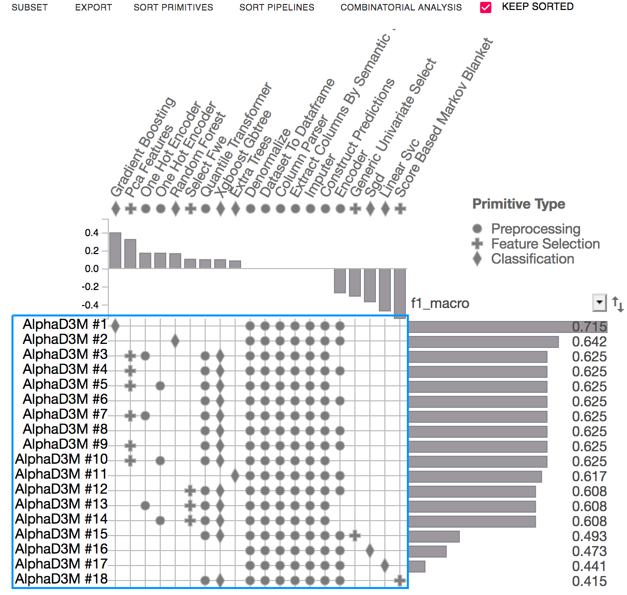
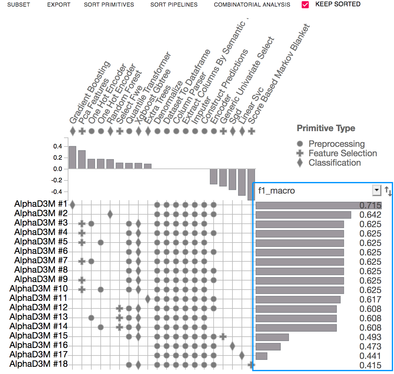
The score view displays performance metrics (i.e. accuracy, F1) of the evaluated pipelines. It can also visualize the training time of each of the pipelines.
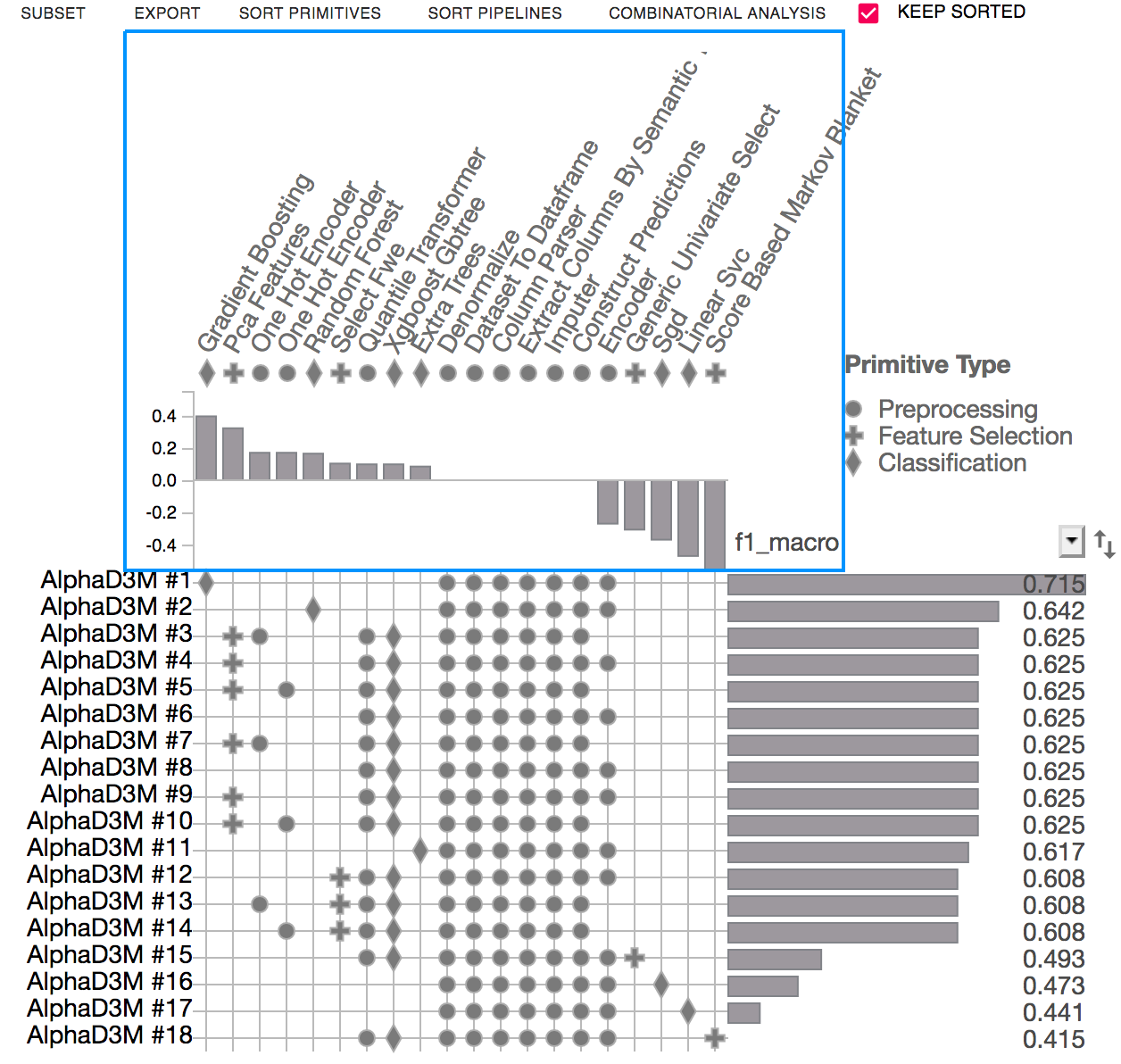
The Primitive Contribution view shows the correlation between primitive usage and the pipeline scores.
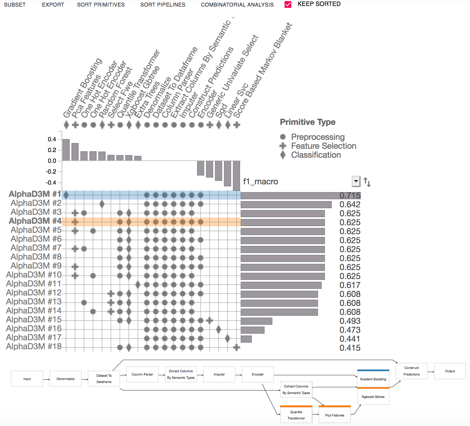
The Pipeline Comparison view highlights the differences between selected pipelines. It presents a node-link representation of the selected pipelines. Multiple pipelines can be selected by shift-clicking the matrix rows.
For more information about how to use PipelineProfiler, click here. There is also a video demo available here.
After the analysis is complete, end the session to clean up temporary files:
[10]:
automl.end_session()
INFO: Ending session...
INFO: Session ended!
Download this example as a jupyter notebook file ( .ipynb ).